Patterns in Palaeontology — Deducing the tree of life

by Russell Garwood*¹

Introduction

“Increasing knowledge leads to triumphant loss of clarity” — Palaeontologist Alfred Romer

Some areas of life and human endeavour have the luxury of certainty. Along these paths of discovery, there are things we can know to be true or false. In others, it is impossible to assess the concept of truth: it can’t be established, or just isn’t a consideration. And between these extremes is a whole mess of important stuff. Palaeontology almost always lies somewhere on this gradation. Researchers studying past life are often juggling multiple layers of uncertainty. We try to balance the need to say something useful — something with meaning, that moves a field and its consensus closer to the truth — with the risk of over-interpreting our data. If the data is too incomplete, we could be moving closer or further away from the truth, and wouldn’t be able to tell. As such, palaeontologists have to draw a line somewhere, and where might differ between people. In other words, palaeontology is very much a human endeavour. It is subject to paradigm shifts in our understanding brought about by new discoveries and methods, but is also influenced by the human nature of those who practise it as fashions and traditions change — normally in search of a better way of doing things. Often, these shifts are driven by arguments that explode onto the scene in which proponents of different ideas — held with passion and fervour — disagree about something harder to pin down and less concrete than a new fossil. This is a position in which palaeontologists who enjoy trying to work out the shape of the tree of life currently find ourselves. Two competing approaches to working out the relationships between different species — their phylogeny — are battling it out in the scientific literature. It’s exciting, engaging and undeniably driven by a desire to improve understanding of the natural world in all its complexity. But it’s also one of those situations in which working out what is closest to the truth can be challenging. Before I write about it any further, we need some context. This article provides both the history of, and current debates surrounding, how we deduce the shape of the tree of life.

From taxonomy to cladistics

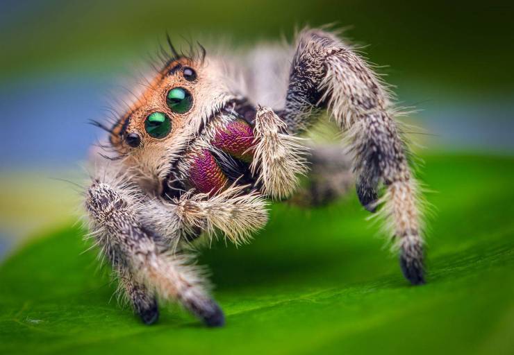
Carl Linnaeus was born in 1707 in Råshult, Sweden. He was a physician and naturalist, working in both botany and zoology. He is now remembered for the system of classification that bears his name. This Linnaean taxonomy gives species a binomial name (sometimes known as a Latin name although not always Latin in origin), and then places them into decreasingly specific levels. So, the beautiful regal jumping spider (figure 1) is Phidippus regius: regius is the species and Phidippus is the genus.

This genus is itself in a family (Salticidae, the jumping spiders), which is in an order (Araneae, the spiders), in a class (Arachnida, which also includes scorpions, mites and a host of other creepy crawlies). That is in the phylum Arthropoda with hexapods (insects and their kin), myriapods (millipedes, centipedes and a couple of other groups), crustaceans (crabs, lobsters, woodlice — and many other collections of mostly marine creatures) and the extinct trilobites. And this is all within the animals (kingdom Animalia).

So far, so good? Well, not quite. This system has been used ever since Linnaeus’s time to categorize all elements of the tree of life, so it is certainly useful. But actually, we can think of the tree of life as a nested series of groups derived from a common ancestor. The animals, for example, have a really deep split between the sponges — which don’t really have tissues or organs — and all other animals. We think (this is actually rather controversial, and another ongoing debate). The rest of the animals can then be broadly split into those without bilateral (two-way) symmetry, and those with it (which typically also have a mouth, anus and through-gut, for example). Those, in turn, can probably be split into two major groups. In fact, every time the tree splits, we get another two groups, which share a common ancestor (a clade, figure 2).

This is a good way of thinking about the tree of life, because it reflects the evolutionary history of all of these groups (which is often — but not always — what people are looking at when they study animals). It is also a really useful way to communicate relationships at a huge variety of levels, whether you’re trying to understand the deepest splits in the animals, in the arachnids or in the spiders. It doesn’t, however, map directly on to Linnaean taxonomy, because every clade — all the way back down to our jumping spider — could have its own name (figure 3), and you can’t split that nested series of groups into a limited number of levels like that of Linnaeus’s scheme.

In response to this, a shift in approach kicked off in the 1960s. As one might expect, there were competing methods: for example, phenetics, which groups organisms by their anatomical similarity, versus schools of thought that focus on the evolutionary history of groups. Although the former approach can be helpful in answering some questions, it was the latter that caught on. German entomologist Willi Hennig was a key figure in this period and in the establishment of classifications that reflect evolutionary history — although the roots of this type of thought lie much deeper. Hennig, born in 1913, published and publicized a scheme that he called phylogenetic systematics. This classifies organisms on the basis of clades that are defined by shared features — such as the through-gut and symmetry of bilaterian animals. This is now commonly referred to as cladistics (although the meaning of this phrase has subtly shifted since it was first coined).

Adding computers to cladistics

Cladistics is an attractive approach for understanding the evolutionary history of a group of organisms, but it is also very challenging if the only tools for building your phylogenies are a pen and paper. People have been visualizing the history life in the form of a tree since before the publication of Charles Darwin’s On The Origin Of Species in 1859, and have done so increasingly since; phylogenetic systematics is a logical extension of this. Traditionally, trees were constructed by studying the organisms to include, then drawing inferences from their anatomy. This is difficult for other researchers to reproduce, and tree shape can result from — or necessitate — a researcher placing particular importance on some elements of a group’s anatomy over others.

These issues have, to an extent, been overcome through the advent and application of powerful modern computers. Researchers generally establish phylogenies for fossils — and, up until the 1990s, commonly living species — by coding their anatomy. You study an animal (or member of any other group) and list what is known as a series of characters: for example, how many eyes they have (for our jumping spider, eight) or the number of legs. It is also possible to include measurements or ratios (called continuous characters). It’s often good to think of characters as a way to test whether two features might be related. As an example, we might code both moths and spiders as capable of making silk — but the many other anatomical differences between these creatures should still keep them in separate groups. With all of this data in hand, we can then try to deduce a tree. We have generally done this since the 1970s using an approach called maximum parsimony, described in glorious and unflinching depth in this Palaeontology [online] article. The basic aim is quite straightforward: to find the trees that require the smallest number of character changes between clades. The underlying principle of maximum parsimony is that the fewer assumptions required, the better (an approach sometimes called Occam’s razor; figure 4).

How this works practically is a tiny bit more complex. The collection of all possible arrangements of trees for a set of species is sometimes referred to as tree space, and we have to search this. We start with a random tree, count the number of changes of characters that it necessitates, then change the tree shape in some way, count again, and repeat until we are confident that we have found the arrangements of groups (whether that be one, or several, trees) that require the least number of character changes. The reason we search like this, rather than trying every possible tree, is that tree space is vast; for twenty species, there are 2.22 × 1020 possible rearrangements. Once you hit 50 species, there are more possible shapes than there are atoms in the Universe. The scale of this task thus calls for computer-based methods.

There are several approaches for searching tree space for those shapes with the smallest number of character changes, but we would hope that they all find the same trees. There can, of course, be multiple trees that imply the same (smallest) number of character changes. In these cases, we summarize them by creating a consensus tree: one which shows all the relationships they agree on, but collapses other relationships (figure 5). This approach of searching tree space and finding the most parsimonious trees has allowed researchers to deduce ever bigger trees (phylogenies) from larger data sets since the 1970s, as tools have developed.

The advantages of cladistics over what came before are that tree searches and their results are reproducible, and that all the assumptions that have gone into building a tree are documented. This is good. But, as before, many researchers believe this approach has imperfections. It is clear from studying the natural world that evolution doesn’t always follow the smallest number of character changes. To choose two examples: snakes evolved from limbed ancestors, rather than those without limbs; and animals have moved from the sea to land (and back again) repeatedly.

Molecules and models

Since the late 1980s, when looking at living organisms, we have been able to use DNA as well as anatomy to deduce their relationships. The principle is similar to that we’ve already seen: DNA is just another form of data, albeit one comprised of sequences of four nucleotides (adenine, thymine, guanine and cytosine). The more closely related organisms are, the more similarities we find in their DNA (in the same way that closely related organisms tend to have similar anatomy). At this molecular level, when species evolve as distinct lineages, they do so through mutations in their DNA, and the longer it has been since two species split (that is, the more distantly related they are), the more mutations will have accrued. Maximum parsimony can struggle here, however. Just as marine reptiles and marine mammals have both evolved to have flippers, despite not being closely related, there are distinct patterns in the changes we see in DNA, which can make sequences start to look alike for distantly related species. This is, in part, because there are just four options at any point in a snippet of DNA, but also because even within one strand, different parts serve very different roles and some don’t really affect the nature of the organism. All this means that using parsimony can start to cluster distantly related species (those on the ends of long branches of the phylogeny, along which lots of DNA mutations have occurred). When this happens, the more molecular data you set to a task, the stronger this incorrect species clustering pattern is. You might ask how we know it is incorrect, but there are normally other lines of evidence pointing towards this mistake when it occurs.

Because of this, researchers creating molecular phylogenies — trees built using DNA — have started using model-based approaches. These have become more common in recent years, in part because computers have become powerful enough to implement them, but also because we can now create a realistic model for how DNA evolves. Model-based approaches come in a number of flavours, but today I want to introduce just one, which has started to be applied to morphology in the past decade. More of that soon. This approach is called Bayesian phylogenetics. It’s named after Thomas Bayes, an English minister and statistician who worked on a theory of probability that eventually took his name — but was actually published by a colleague, on the basis of Bayes’ notes, after his death. Bayes’ theorem, in its simplest form, allows us to deduce the probability of something — say, an event, or the shape of an evolutionary tree — given prior knowledge of the conditions related to it. In the case of the tree, this knowledge could be the sequences of DNA from the species in a phylogeny, and a model of how their nucleobases change. This amounts to the probability over time of switches between any of the nucleobases — something that can be mapped (or modelled) on to a tree shape, and the probability of that tree can then be quantified. This is called the posterior probability. The next obvious question is, how do we actually use this to derive a tree? Well, that’s achieved using an algorithm called a Markov chain Monte Carlo (MCMC), which samples the posterior-probability distribution of possible trees.

Let’s break this down and explain what that actually means. To do so, we have to consider changing the trees — the relationships and length of branches (the amount of change that has occurred along them). This gives us a space we can explore that might be best imagined as a rugged, mountainous landscape. The x and y coordinates of this space — the position on a map of the terrain — could be thought of as the tree shape, and the height of the landscape is the posterior probability of the trees at that point given the data and the model of evolution. An MCMC analysis explores this landscape: it starts from a random place, and repeatedly changes the tree. It then accepts a new tree if its posterior probability is higher, or a little lower, than the previous one (that is, the change from the last tree allows the analysis to climb up one of our imaginary mountains or stay about level). If the posterior probability of a tree is much lower than what came before (that is, it takes us downhill), then the MCMC discards that tree, and sticks with the previous one. This process is then repeated, hundreds of thousands to millions of time.

Eventually, by doing this, the algorithm reaches an equilibrium: it is just wandering around the same area over and over again, and visiting the higher area more often (in fact, how often it visits each area is proportional to their posterior probability; figure 6). Thus, our route over this landscape represents the most probable trees, but also takes into account uncertainty in the data. If we take all of the trees we’re wandering over, and create a summary of them, this is a good way of deriving the relationships between species given their data and our model of evolution, while incorporating uncertainty. It’s a well-established approach when using DNA, and is widely used to work out the relationships between living species.

Morphology and models

So why — I am sure you are wondering by this point — have I subjected you to all of this hardcore phylogenetics in an article for Palaeontology [online]? It’s because in recent years, these methods have started to have an impact on palaeontology. We can’t recover the DNA of fossils so, to use Bayesian approaches on extinct organisms, we need a model for the evolution of anatomy. This will let us work out the posterior probability of a tree given morphological character data (the same data that we might have gathered for a parsimony-based analysis). Now, this is pretty tough, and currently for morphological Bayesian phylogenetic analyses we use something called the Lewis or MK model, in which switches between any character states (in any direction) are equally likely. This is an assumption, but it does allow Bayesian MCMC approaches to be used for fossils. Fossils often lack data, and so using Bayesian analysis is quite attractive, because it incorporates uncertainty — we can think of it, perhaps, as a slightly more cautious way of deriving a tree. It has a few other benefits, as well. But then we get to another tricky problem: how do we actually assess which approach is better, parsimony or Bayesian? We don’t have the true tree to check them against (otherwise we wouldn’t need to do this), and DNA-based analyses have their own potential issues, so we can’t necessarily treat those as correct.

The past few years have been exciting in the world of morphology and phylogenetics because a slew of papers have used simulations to ask this very question. Simulations allow us to take a tree and generate data that reflects its shape. In this situation, we have both the true tree and data that reflects it. If we use the data and parsimony, Bayesian and other approaches to try to reconstruct the tree, we can compare the derived tree with the truth — and ultimately work out which way of building trees is better. We hope. But the devil is always in the details, and it turns out that researchers have impassioned views about which approach should be used, so there has been a heated debate. A series of papers have used more and more complex models of molecular evolution (increasingly far removed from the Lewis model of morphological evolution) to generate data onto trees — see the papers led by Wright, O’Reilly or Puttick in Further Reading. These articles have shown that Bayesian phylogenetics has an edge over parsimony (figure 7): the take-home message has been that parsimony-based methods are less accurate than Bayesian (they are more different from the true tree), but also that parsimony methods are more precise (they resolve more relationships in general — but of course, that’s not particularly useful if those relationships are not correct!).

This suggests that palaeontologists should build their trees using Bayesian inference. But enter parsimony proponents. Argentinian arachnologist and parsimony-software developer Pablo Goloboff and his colleagues have penned replies to the above papers, calling into question their narrative. One thrust of the argument is that the models used to generate data (and then deduce trees to compare methods) favour Bayesian over parsimony. Adding spice to the mix is the suggestion that the methods used to compare the similarity of derived and true trees are also very sensitive to particular types of difference, and that more methods should be used. This debate is continuing — the authors of the earlier papers have responded to the criticisms, and while I have been writing this very article a new paper from Pablo Goloboff has appeared highlighting the lack of realism of the Lewis model of morphological evolution. What does this all mean? Unfulfilling as it is, I don’t think there is a conclusion in sight — yet. But I think this situation does allow us to make some interesting observations about how we do science.

Human nature and science

A really interesting factor in all of this is how very human everything is getting — not surprising given that researchers are humans, but an excellent illustration of how science may strive for objectivity, but other forces remain in play. In science, as in other human endeavours, cliques and fashions can develop and disappear, and everything is swayed by human nature. This is especially noticeable in an episode such as this, where differences are subtle and truth is hard to pin down. One outcome is that strong opinions form, and the defence of a preferred technique can become impassioned. As an example, the Goloboff et al. (2017) paper contains some remarkably strongly worded statements. One is:

Although they generated their data sets with models specifically chosen to make Bayesian methods perform better  than parsimony, Wright and Hillis (2014), O’Reilly et al. (2016) and Puttick et al. (2017) asserted, with typical grandiloquence, that Bayesian methods are superior to parsimony in general.

The contents of this statement can be debated, yet you wouldn’t guess that from the words.

And all this is taking place in a community of researchers, which will affect what happens now. While arguments are raging in some circles, others are marked by inertia. Changing how people infer trees necessitates teaching them new techniques. It requires ‘traditional’ approaches to be abandoned, and researchers must reassess the body of knowledge that we have built on top of the relationships constructed using parsimony. It could be that Bayesian techniques will not resolve some relationships at all. If this is the case, is it better to have some hypothesis to test when new fossils are discovered, constructed using parsimony but potentially wrong, or is it best to conclude that we just don’t have enough data yet? Add to this dilemma the fact that Bayesian versus parsimony doesn’t have a cut and dried answer. You then have the question of when would or should we make the switch to mainly using Bayesian — how certain do we need to be that it is better? Will there be a parallel of the cladistics takeover for Bayesian? Or will this all fizzle out if we can’t work out which approach is better?

I don’t have any answers to these questions, but it certainly makes trying to work out the relationships between extinct species an exciting and rapidly developing field right now. So, in lieu of answering these questions — because I can’t — I will finish with some personal thoughts. At the moment, we don’t have a clear-cut winner when it comes to reconstructing evolutionary relationships using anatomy. Until we do, perhaps a good approach would be to use both methods: if they agree, then we can probably have some confidence in the relationships they infer. If they don’t, then we know that there may be a weak signal in the data we are using, and further work needs to be done. If we settle on one technique down the line, then future readers can place more weight on its results. But above and beyond this, the key uncertainty in both simulation studies and model-based approaches to building evolutionary trees is our lack of a clear model of how anatomy evolves in the real world. With better models for the evolution of morphology, we can both simulate better data to test inference techniques, and derive better trees from real-world data. I think this is where our efforts might be best placed. We know evolution isn’t parsimonious: it doesn’t follow the simplest path. So ultimately, with better models for morphological evolution, we should be able to build better trees using Bayesian than using parsimony. But we are not there yet — not even close. There is lots still to be done. That’s not an awful place to be, because, damn, it’s exciting.

Suggestions for further reading

Goloboff, P. A., Torres, A. & Arias, J. S. Weighted parsimony outperforms other methods of phylogenetic inference under models appropriate for morphology. Cladistics 34, 407–437 (2018). DOI: 10.1111/cla.12205

Goloboff, P. A., Torres Galvis, A. & Arias, J. S. Parsimony and model‐based phylogenetic methods for morphological data: comments on O’Reilly et al. Palaeontology 61, 625–630 (2018). DOI: 10.1111/pala.12353

O’Reilly, J. E., Puttick, M. N., Parry, L., Tanner, A. R., Tarver, J. E., Fleming, J., Pisani, D. & Donoghue, P. C. Bayesian methods outperform parsimony but at the expense of precision in the estimation of phylogeny from discrete morphological data. Biology Letters, 12, 20160081 (2016). DOI: 10.1098/rsbl.2016.0081

O’Reilly, J. E., Puttick, M. N., Pisani, D. & Donoghue, P. C. Empirical realism of simulated data is more important than the model used to generate it: a reply to Goloboff et al. Palaeontology  61, 631–635 (2018). DOI: 10.1111/pala.12361

Puttick, M. N., O’Reilly, J. E., Tanner, A. R., Fleming, J. F., Clark, J., Holloway, L., Lozano-Fernandez, J., Parry, L. A., Tarver, J. E., Pisani, D. & Donoghue, P. C. Uncertain-tree: discriminating among competing approaches to the phylogenetic analysis of phenotype data. Proceedings of the Royal Society B 284, 20162290 (2017). DOI: 10.1098/rspb.2016.2290

Wright, A. M. and Hillis, D. M. Bayesian analysis using a simple likelihood model outperforms parsimony for estimation of phylogeny from discrete morphological data. PLoS One 9, e109210 (2014). DOI: 10.1371/journal.pone.0109210

 

---

¹ School of Earth and Environmental Sciences, University of Manchester, Manchester M13 9PL, UK